


Here at Vertica, we had to solve a technical challenge that many of you might be facing: data analysis from legacy products. When a customer reports an issue to customer support, we commonly ask for a diagnostic dump. This dump contains structured event data on what the database was doing at the time the problem occurred and provides a primary source of information for resolving the customer’s issue. The dump contains a collection of tables, written out in a simple delimited format similar to the output of a ‘SELECT * from T’ statement. Since the data size can be quite large (gigabytes), we load it into a (ha-ha) Vertica database for analysis. The complication is that the contents of this diagnostic dump vary by Vertica version. We therefore needed a way to ingest the data and make use of it despite the schema varying based on the source version.
A mostly-fixed but time-varying schema is a great use case for the newly released Vertica 7 (aka Crane) flex tables feature. With flex tables, we can load the data without fully defining the schema and query the part of the data we need. Indeed, reading our own diagnostic data was the first serious use of flex tables and served to refine our design for the feature. In this post, we will walk you through capturing, loading, and querying data from Vertica’s own DataCollector (DC) tables using Vertica’s flex tables. While previous posts have focused on loading JSON data, Vertica Flex tables support a number of different input formats, including delimited data.
A Whirlwind Tour of the DataCollector
Vertica’s Data Collector is our mechanism for capturing historical event data for internal database reporting and diagnostic analysis. Many of our system tables that display historical information, such as query_requests or load_streams, are actually views built on top of data collector tables. Because they change frequently and can be opaque to users outside of Vertica, we don’t document them. If you want to muck around, take a look at:
select data_collector_help();In this example, we examine a couple of tables that track transactions on the Vertica cluster, the first of which is called DC_TRANSACTION_ENDS. This table has a row for every transaction that completes on each node in the cluster:
select * from dc_transaction_ends limit 4;

time | node_name | session_id | user_id | user_name | transaction_id | number_of_statements | is_committed | end_begin_time | epoch_close_time | end_epoch | is_ddl | ros_rows_written | dvros_rows_written | wos_rows_written | dvwos_rows_written

2014-01-22 00:32:08.025521-05 | initiator | localhost.localdoma-10040:0xb | 45035996273704962 | bvandiver | 45035996273704963 | 1 | t | 2014-01-22 00:32:08.016667-05 | | 1 | t | 0 | 0 | 0 | 0

2014-01-22 00:32:08.03535-05 | initiator | localhost.localdoma-10040:0xb | 45035996273704962 | bvandiver | 45035996273704964 | 1 | f | 2014-01-22 00:32:08.03491-05 | | 1 | t | 0 | 0 | 0 | 0

2014-01-22 00:32:09.163234-05 | initiator | localhost.localdoma-10040:0xf | 45035996273704962 | bvandiver | 45035996273704965 | 1 | f | 2014-01-22 00:32:09.163122-05 | | 1 | t | 0 | 0 | 0 | 0

2014-01-22 00:32:09.175018-05 | initiator | localhost.localdoma-10040:0xf | 45035996273704962 | bvandiver | 45035996273704966 | 1 | f | 2014-01-22 00:32:09.174786-05 | | 1 | t | 0 | 0 | 0 | 0
Queries against this table can reveal a number of interesting properties of the database workload, such as commit rate, rows per bulk load, DDL percentages, and so on. A companion table called DC_TRANSACTION_STARTS registers a row for each transaction that starts ? it contains less interesting information because the database does not yet know the contents of the transaction. However, joining the two tables tells us the duration of each transaction.
Capturing a Data Dump
The simplest possible way to export the data is merely to capture the output of running a SQL query ? and indeed we frequently need to consume this ad hoc format here at Vertica. From within vsql, Vertica’s command line client, you can do this with:
bvandiver=> aWe switch to unaligned output to avoid dumping a huge number of useless blank spaces into the output. An alternative is to merely capture the output with shell redirect:
Output format is unaligned.
bvandiver=> o /tmp/dce.txt
bvandiver=> select * from dc_transaction_ends;
bvandiver=> o
/opt/vertica/bin/vsql -A -c "select * from dc_transaction_ends;" > /tmp/dce.txtThe contents of the file will look something like this:
time|node_name|session_id|user_id|user_name|transaction_id|number_of_statements|is_committed|end_begin_time|epoch_close_time|end_epoch|is_ddl|ros_rows_written|dvros_rows_written|wos_rows_written|dvwos_rows_written

2014-01-22 00:32:08.002989-05|initiator|localhost.localdoma-10040:0x3|45035996273704962|bvandiver|45035996273704961|1|f|2014-01-22 00:32:08.002313-05||1|f|0|0|0|0

2014-01-22 00:32:08.009437-05|initiator|localhost.localdoma-10040:0x3|45035996273704962|bvandiver|45035996273704962|1|t|2014-01-22 00:32:08.008547-05||1|f|0|0|0|0

2014-01-22 00:32:08.025521-05|initiator|localhost.localdoma-10040:0xb|45035996273704962|bvandiver|45035996273704963|1|t|2014-01-22 00:32:08.016667-05||1|t|0|0|0|0

2014-01-22 00:32:08.03535-05|initiator|localhost.localdoma-10040:0xb|45035996273704962|bvandiver|45035996273704964|1|f|2014-01-22 00:32:08.03491-05||1|t|0|0|0|0

2014-01-22 00:32:09.163234-05|initiator|localhost.localdoma-10040:0xf|45035996273704962|bvandiver|45035996273704965|1|f|2014-01-22 00:32:09.163122-05||1|t|0|0|0|0

2014-01-22 00:32:09.175018-05|initiator|localhost.localdoma-10040:0xf|45035996273704962|bvandiver|45035996273704966|1|f|2014-01-22 00:32:09.174
Exploring the data
How would you load this data into a regular SQL database? Well, you’d have to look at the input file, determine the column count and types, write a large CREATE TABLE statement, and then bulk load the data. With Vertica’s flex tables, you need to do only the following:
CREATE FLEX TABLE dce();The FDelimitedParser is a flexible parser much akin to Vertica’s regular COPY parser. The delimiter defaults to ‘|’, which is why it need not be specified here (3 guesses why we picked that default…). Flex tables make it really easy to get the data into the database ? something that comes in handy when customers are anxiously awaiting diagnosis! Since we never had to describe the schema, no matter which version of Vertica supplied the source data, the load still completes successfully.
COPY dce FROM '/tmp/dce.txt' PARSER FDelimitedParser();
Queries are equally straightforward. Just pretend the columns exist! The following query shows the transactions that wrote the largest number of rows:
Query 1:
select sum(ros_rows_written + wos_rows_written) from dce group by transaction_id order by 1 desc limit 10;Alternatively, this query computes commits per second over the interval captured
select sum(ros_rows_written + wos_rows_written) from dce group by transaction_id order by 1 desc limit 10;Queries are equally easy – just pretend the columns exist! The following query shows the transactions that wrote the largest number of rows:
Query 2
select sum(ros_rows_written + wos_rows_written) from dce group by transaction_id order by 1 desc limit 10;Alternatively, this query computes commits per second over the interval captured:
select count(time) / datediff(ss,min(time::timestamp),max(time::timestamp)) from dce where is_committed = 't';Much like many NoSQL solutions, flex tables require the type information to be supplied at query time, in this case in the form of casting the time column to a timestamp. In many cases, automatic casting rules convert the base varchar type to something appropriate, such as the sum() above casting its inputs to integers. You are not limited to trivial SQL, for example you can load DC_TRANSACTION_STARTS and join the two tables to compute average transaction duration:
Query 3:
select avg(ends.end_time - starts.start_time) fromThis query needs the subqueries because a row for every transaction exists on every participating node and we want to find the earliest and latest entry. When joining flex tables, you need to fully qualify all source columns with their originating table because either table could possibly have any column name you supply! To simplify, you can have Vertica build a view for you:
(select transaction_id,max(time::timestamp) as end_time from dce group by transaction_id) ends,
(select transaction_id,min(time::timestamp) as start_time from dcs group by transaction_id) starts
where ends.transaction_id = starts.transaction_id;
select compute_flextable_keys_and_build_view('dce');Querying the view dce_view looks very much like querying the original Data Collector table. In fact, any of the SQL we just wrote against the flex tables is valid when run against the original source tables DC_TRANSACTION_ENDS and DC_TRANSACTION_STARTS! Accessing flex tables is identical to accessing regular tables–a true illustration of how flex tables meet the underlying promise of SQL databases. Users do not have to know the underlying data storage to derive value from the data.
In search of performance
We get some really large diagnostic dumps and can’t always afford the performance degradation of unoptimized flex tables. Improving performance is particularly simple for tables from the Data Collector because we know upfront which columns are important predicate and join columns. Furthermore, these columns are present in most DC tables and are unlikely to vary. Thus, we use a hybrid flex table: specify some important columns and let the rest of the hang out in the “Flex Zone”. We use the following definition for most DC tables:
CREATE FLEX TABLE hybrid (In our performance evaluation shown in Figure 1, we compare running the above queries using an unoptimized flex table with no explicit columns against an optimized flex table with explicit columns. The optimized tables have same columns, sort order, and segmentation of the “hybrid” table shown above and the experiment was run on 3 virtual machines hosted on an HP DL380 with 12 cores and 96GB of RAM. On the optimized table, Query 1 is an aggregation over an explicit column which appears in the sort order, leading to an efficient aggregation mechanism. Query 2 has a selective predicate column which is not explicit in the optimized table and thus doesn’t gain significant benefit. Query 3 derives significant benefit because the join columns are explicitly part of the sort order and segmentation expression for the optimized table, leading to a cluster aware join which is very memory efficient. With our optimized table, we get the best of both worlds: speedy queries and flexible schema.
time timestamptz,
node_name varchar(100),
session_id varchar(100),
user_id int,
user_name varchar(100),
transaction_id int,
statement_id int,
request_id int
) order by transaction_id,statement_id,time segmented by hash(transaction_id) all nodes ksafe 1;
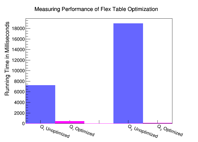
Figure 1: Performance comparison of sample queries run on the unoptimized flex table versus the optimized hybrid flex table. Query 1 is a simple aggregate query and Query 3 is a simple join. The graph shows that optimization sped up Query 1 by a factor of 17, and Query 3 by a factor of 121.
And in conclusion
Flex tables have changed our ingest logic from a complicated and brittle collection of static scripts to one simple Python script that handles it all. And I am much more willing to accept general query dumps from customers, since even if they are 300 columns wide I can still trivially pull them into Vertica for analysis. It all works because flex tables are not just about supporting JSON in the database, they are about changing the way we store and explore data in a relational database.
About the Author
Ben Vandiver