Estimate the Price of Diamonds Using Vertica Machine Learning

This blog post was authored by Vincent Xu.

In this blog post, I’ll take you through the exercise I did to estimate the price of a diamond based on its characteristics, using the linear regression algorithm in Vertica. Besides Vertica 9.0, I used Tableau for charting and DbVisualizer as the SQL editor. From this exercise, I hope you’ll see how easy and natural it is to conduct machine learning using the tool set that business analysts already have.

The data set used in this post is from Kaggle. For convenience, the dataset, SQL notebook and Tableau workbook are available on Github. Feel free to install a free version of Vertica, DbVisualizer and Tableau, if you don’t have them, and run the exercise by yourself.

Explore the Data

To start, let’s examine the dataset. The dataset is loaded into the ‘diamond’ table in Vertica. SQL and a rich set of Vertica built-in functions allow you to slice and dice the data however you want. From here on, I call properties features.

The table has 11 columns. Categorical features include:

1. id – unique identifier of the 53,940 diamond samples
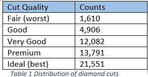
2. cut – quality of the cut



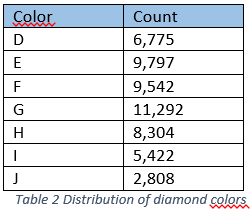
3. color – color of the diamond



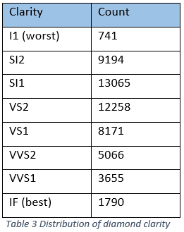
4. clarity – measurement of diamond clarity



Numerical features include:

5. price – price in US dollars
6. carat – weight of the diamond
7. X – length in mm
8. y – width in mm
9. z – depth in mm
10. depth – depth percentage = z / mean(x, y) = 2 * z / (x + y); its column is named ‘depthh’ to avoid conflict with SQL reserved words
11. table – width of top of the diamond relative to its widest point; its column is named ‘tablee’ to avoid conflict with SQL reserved words

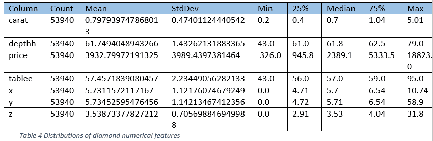
Run the summary function to get distribution of these features: => SELECT SUMMARIZE NUM_COL (price, carat, x, y, z, depthh, tablee) OVER() FROM diamond;

Transform the features

1. Create dummy features for the categorical features.

The categorical features ‘cut’, ‘color’ and ‘clarity’ need to be converted to numerical features before they can be fed into the linear regression training function. ‘cut’ and ‘clarity’ are ordinal data and may be converted to numbers such as 1, 2 and 3, etc. However, the distance between each level is hard to quantify. In my experiment, they are all converted into dummy features. => SELECT ONE_HOT_ENCODER_FIT ('diamond_onehot', 'diamond_sample', 'cut,color,clarity'); The function ‘one_hot_encoder_fit’ analyses all the values in each of the specified columns and stores the result in the model ‘diamond_onehot’. The input table ‘diamond_sample’ contains all the columns from ‘diamond’ with the addition of a couple columns. One such added column is ‘part’, which labels each sample as ‘train’ or ‘test’ randomly. 70% percent of samples are used for training and 30% for testing.

You can examine categorical levels for each column contained in the model by running the command: => SELECT GET_MODEL_ATTRIBUTE (USING PARAMETERS model_name='diamond_onehot', attr_name='varchar_categories'); The following command applies the model to the dataset, generates the dummy columns and stores them in the table ‘diamond_encoded’. => CREATE TABLE diamond_encoded as (SELECT APPLY_ONE_HOT_ENCODER (*USING PARAMETERS model_name='diamond_onehot', drop_first='true') FROM diamond_sample); By specifying “drop_first=’true’”, the function generates one less dummy column than the number of distinct values in the original column, because the extra dummy column is redundant. Looking into the table ‘diamond_encoded’, you’ll find these dummy columns:

• cut_1, cut_2, cut_3, cut_4
• color_1, color_2, color_3, color_4, color_5, color_6
• clarity_1, clarity_2, clarity_3, clarity_4, clarity_5, clarity_6, clarity_7

2. Normalized the numerical predictors

It’s a good practice to normalize the predictors, especially when regularization is used. => SELECT NORMALIZE ('diamond_normalized', 'diamond_encoded', 'carat,logcarat,depthh,tablee,x,y,z', 'robust_zscore'); And you can see the resulting values for each predictor all have similar ranges.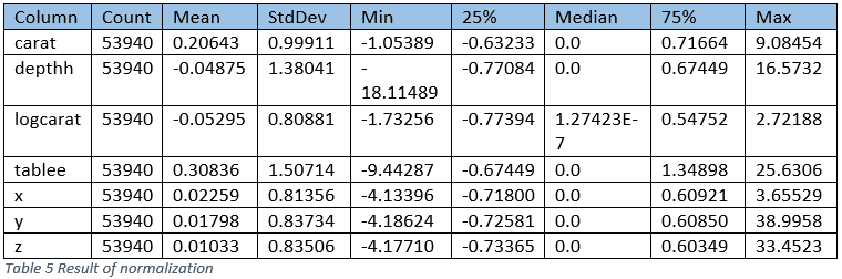



3. Create the training and testing datasets

Since we will train models repeatedly, let’s materialize the view and store the training and testing data in table ‘diamond_train’ and ‘diamond_test’, respectively. => CREATE TABLE diamond_train AS SELECT * FROM diamond_normalized WHERE part='train'; => CREATE TABLE diamond_test AS SELECT * FROM diamond_normalized WHERE part='test';

Build the Model

Now that we have the data prepared, we will experiment with modelling to see how well we can make the model estimate the price of a diamond. We’ll start with a simple model, observe it, and find ways to improve it.

1. Model 1 – build a linear-regression model using price as the response variable.

Run the training with all the features, except ‘id’ and ‘price’, as predictors. It takes about a second or two to finish. The resulting model is saved in Vertica as ‘diamond_linear_price’. => SELECT LINEAR_REG ('diamond_linear_price', 'diamond_train', 'price', 'carat, cut_1, cut_2, cut_3, cut_4, color_1, color_2, color_3, color_4, color_5, color_6, clarity_1, clarity_2, clarity_3, clarity_4, clarity_5, clarity_6, clarity_7, depthh, tablee, x, y, z'); And run the prediction on the testing dataset: => CREATE TABLE pred_linear_price AS (SELECT id, price, predict_linear_reg (carat, cut_1, cut_2, cut_3, cut_4, color_1, color_2, color_3, color_4, color_5, color_6, clarity_1, clarity_2, clarity_3, clarity_4, clarity_5, clarity_6, clarity_7, depthh, tablee, x, y, z USING PARAMETERS model_name = 'diamond_linear_price') AS prediction FROM diamond_test); The prediction result is saved to table ‘pred_linear_price’. We can evaluate the model by calculating mse, rsquared, and correlation based on the prediction result. => SELECT MSE (price, prediction) OVER() FROM pred_linear_price; 1268641.9733099 => SELECT RSQUARED (price, prediction) OVER() FROM pred_linear_price; 0.919810051437739 => SELECT CORR (price, prediction) FROM pred_linear_price; 0.959093103572715 We can visualize the predicted price vs. the actual price. The result is not too bad, but we can see much can be improved. Many of the predicted prices are negative.



2. Model 2 – build the model with log(price)

For diamonds, the size of the diamond should affect its price greatly based on our experience. Let’s examine size more closely by plotting it against price. From the chart below, we can see the relationship between these two is somewhat exponential. Price sensitivity exhibits exponential pattern commonly in real life.



To make the price-carat relation more linear, let’s take a 10-based logarithm of the price and use it as the response variable instead. We run a similar training command as we did previously, create the model, and run the prediction on the testing data set. The chart below plots the predicted price vs. the actual price.



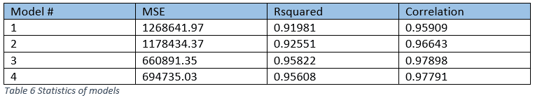
The chart looks much improved. There are no more negative prices, and the following table shows Model 2 improved over Model 1 on all three metrics. Can we improve further from here?



3. Model 3- build a model with log(price) and log(carat)

If we further examine the relationship between log(price) and carat, we’ll notice it exhibits an exponential pattern in the other direction.



How about we take a log of ‘carat’ too? The chart below shows a pretty good linear relationship between these two.



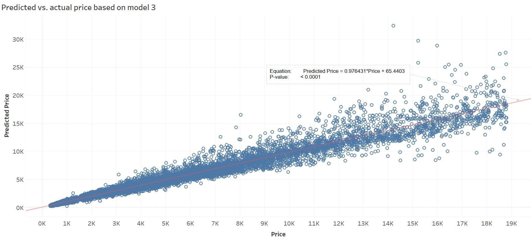
So let’s replace the feature ‘carat’ with log(‘carat’) and keep all other features the same as those of Model 2. The following chart visualizes the predicted price based on Model 3. All the evaluation metrics show further improvements over Models 1 and 2 (see Table 6).



At last, take a look at the parameters of Model 3: => SELECT GET_MODEL_ATTRIBUTE (USING PARAMETERS model_name='diamond_linear_logprice_logcarat', attr_name='details');

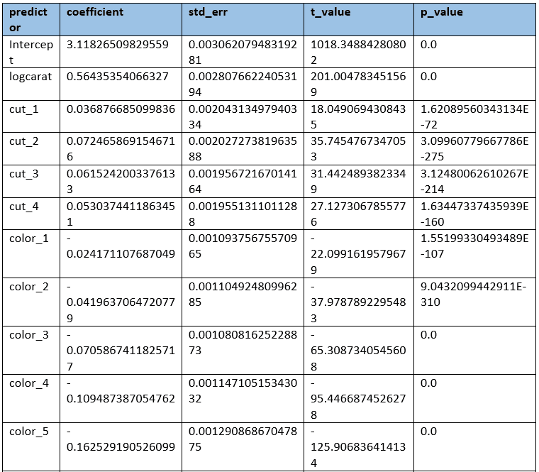
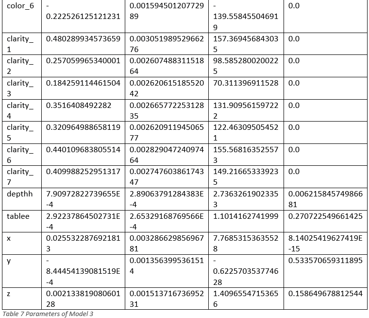
In the table above, we can see ‘tablee’, ‘x’ and ‘y’ have a relatively large p_value and small t_value, which indicates these features are likely not correlated to the price. That leads to regularization.

4. Model 4- Add regularization to Model 3

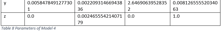
Regularization helps prevent overfitting and even simplifies the model by selecting the relevant features. Let’s apply L1 regularization based on Model 3. => SELECT LINEAR_REG ('diamond_linear_logprice_logcarat_l1', 'diamond_train', 'logprice', 'logcarat, cut_1, cut_2, cut_3, cut_4, color_1, color_2, color_3, color_4, color_5, color_6, clarity_1, clarity_2, clarity_3, clarity_4, clarity_5, clarity_6, clarity_7, depthh, tablee, x, y, z' USING PARAMETERS regularization='l1', lambda=0.005); The lambda value can be adjusted to reflect the level of regularization. With a lambda value of 0.005, the coefficients of 10 predictors have become zero (see table below). As shown in Table 6, Model 4’s performance has only degraded slightly with 10 fewer predictors.

Summary

Before this blog post gets too long, I will claim mission accomplished. More improvements can be made. For example, one thing that is obvious from the chart that shows predicted price vs. the actual price based on model 3 is that the predicted price tends to diverge from the actual price for higher prices. Residual plots can be made to examine the pattern between the price and individual predictor more closely.

Throughout this exercise, Vertica, DbVisualizer, and Tableau have worked seamlessly together. Vertica MPP computing infrastructure makes machine learning run blazingly fast, BI tools’ sophisticated reporting capability makes it a breeze to visualize the results, and DbVisualizer naturally captures the workflow and manages the workflow conveniently. If you’ve been using Vertica and any of the popular BI tools, you already have all the tools to start using machine learning!