


NOTE: This article refers to Vertica 7.x and is considered outdated. This article is more relevant to later Vertica versions.
New in Vertica 7.2.2 is the Machine Learning for Predictive Analytics package. This analytics package allows you to use built-in machine learning algorithms on data in your Vertica database.
Machine learning algorithms are extremely valuable in data analytics because, as their name suggests, they can learn from your data and provide information about deductive and predictive outcomes.
Specifically, you can:
• Pre-process your data with data normalization methods and all other Vertica functions
• Use k-means algorithms for cluster analysis
• Create predictive models using linear and logistical regression algorithms
• Evaluate the accuracy and effectiveness of your models using evaluation functions
In this blog, we’ll go over the following popular machine learning algorithms and accompanying functions:
• kmeans: kmeans(), summaryKmeans(), kmeansApply()
• logistic regression: logisticReg (), summaryLogisticReg(), predictLogisticReg()
• linear regression: linearReg(), summaryLinearReg(), predictLinearReg()
These functions are all available in the v_ml schema when you install the Vertica Advanced Analytics Package, which is included in the Vertica rpm.
You can learn about data normalization and model evaluation in the Vertica documentation.
Clustering Data with the k-means Algorithm
The k-means algorithm is a type of unsupervised learning algorithm. The algorithm takes data and partitions it into k different clusters, based on similarities between the data points.
For example, say you have a small data set called myKMeansTable that lists information about food, including an identification number(ID), sugar content, calories, and category:
=> SELECT * FROM myKMeansTable;
 ID | sugar_content | calories | food_category
----+---------------+----------+---------------
  1 |           0.1 |      0.4 | Fruit
  2 |           0.5 |      0.4 | Fruit
  3 |           0.8 |     0.25 | Fruit
  4 |           0.2 |    0.375 | Vegetable
  5 |           0.5 |      0.5 | Vegetable
  6 |           0.1 |    0.125 | Vegetable
  7 |           0.2 |     0.98 | Bread
  8 |          0.54 |     0.25 | Dairy
  9 |           0.8 |      0.5 | Egg
 10 |           0.1 |     0.75 | Meat
 11 |           0.3 |     0.45 | Dessert
 12 |           0.2 |    0.367 | Dessert
 13 |           0.8 |     0.75 | Bread
 14 |           0.5 |     0.75 | Dairy
 15 |           0.2 |     0.12 | Breakfast
 16 |           0.7 |     0.75 | Vegetable
 17 |           0.6 |    0.625 | Fruit
 18 |           0.2 |      0.5 | Bread
 19 |           0.8 |     0.95 | Dessert
 20 |           0.2 |      0.8 | Dairy

(20 rows)
Here’s how the kmeans function can help you gain insight into your data.
The function creates a model called model_name based on the specified columns (input_columns) of the input data(input_table) that contains centers of detected clusters. The desired number of clustered is specified by an input argument called num_cluster.
kmeans() syntax:
kmeans( ‘model_name’, ‘input_table’, ‘input_columns’, num_clusters[,--parameter_options…])
Example:
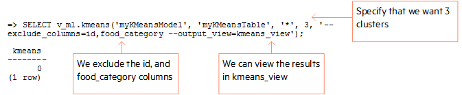
Say you want to cluster the foods into 3 clusters. The following example shows how you can use the kmeans function to create a k-means model called myKmeansModel and view the results of the model in the output_view. Since the algorithm works only on numeric values, we include the category column in the –exclude_columns parameter. We also want to exclude the id, because we don’t need to consider that value when creating clusters. (For a full list of parameters options, see the documentation).
=> SELECT * FROM kmeans_view ORDER BY cluster_id;
 sugar_content | calories | cluster_id
---------------+----------+------------
           0.5 |      0.4 |          0
           0.8 |     0.25 |          0
           0.5 |      0.5 |          0
           0.1 |    0.125 |          0
          0.54 |     0.25 |          0
           0.2 |     0.12 |          0
           0.1 |      0.4 |          1
           0.2 |    0.375 |          1
           0.2 |     0.98 |          1
           0.2 |    0.367 |          1
           0.1 |     0.75 |          1
           0.3 |     0.45 |          1
           0.2 |      0.5 |          1
           0.2 |      0.8 |          1
           0.8 |      0.5 |          2
           0.8 |     0.75 |          2
           0.5 |     0.75 |          2
           0.6 |    0.625 |          2
           0.8 |     0.95 |          2
           0.7 |     0.75 |          2
(20 rows)
As you can see, the data was split up into three groups (clusters).
Predictive Modeling with Logistic and Linear Regression
Unlike the deductive qualities of the k-means algorithm, predictive models are inductive and examples of supervised learning algorithms. This means observed samples are used to train a model, and the resulting model is used to predict future outcomes.
Vertica provides two predictive modeling learning algorithms: logistic and linear.
Logistic Regression
Logistic regression algorithms are used for binary classification purposes. For example, your company may want to analyze how a student’s GPA, SAT score, and club affiliations affect whether or not they are interviewed for a job. In the next couple sections, we’ll show you how to use logistic regression to do so.
Create training data
First, we create a training table that is a subset of our overall data set. This myLogTrainTable includes a student identification number (ID), independent variables, or predictors (GPA, SAT score, number of club affiliations) and a dependent, binary value (interviewed = 1, not interviewed = 0):
=> SELECT * FROM myLogTrainTable;
 ID | GPA | SAT  | clubs | interviewed
----+-----+------+-------+------------
  1 | 3.5 | 1596 |     2 |     1
  2 | 4.1 | 1600 |     1 |     1
  3 | 2.6 | 1400 |     0 |     0
  4 |   3 | 1356 |     3 |     0
  5 | 2.8 | 1256 |     3 |     0
  6 |   4 | 1598 |     0 |     1
  7 | 3.9 | 1566 |     5 |     1
  8 | 2.7 | 1300 |     2 |     0
  9 | 3.3 | 1520 |     3 |     0
 10 |   4 | 1600 |     2 |     1
 11 | 3.2 | 1540 |     0 |     0
 12 | 2.8 | 1350 |     3 |     0
 13 |   4 | 1600 |     2 |     1
 14 | 3.4 | 1542 |     1 |     0
 15 | 3.9 | 1596 |     3 |     1
 16 | 2.9 | 1366 |     2 |     0
 17 | 3.5 | 1555 |     0 |     0
 18 |   4 | 1559 |     1 |     1
 19 |   4 | 1598 |     1 |     1
 20 | 3.6 | 1600 |     2 |     1
(20 rows)
Build model
Then, use the logisticReg function to build a model based on the training data:
logisticReg syntax:
logisticReg ( 'model_name', 'input_table', 'response_column', 'predictor_col1, predictor_col2, ..., predictor_coln', [,--parameter_options…])

=> SELECT v_ml.logisticReg('logisticRegModel', 'myLogTrainTable', 'interviewed', 'GPA,SAT,clubs');
 logisticReg
-------------
           0
(1 row)
View model
View the model’s summary with the summaryLogisticReg function:
=> SELECT v_ml.summaryLogisticReg (USING PARAMETERS owner='dbadmin', model_name='logisticRegModel');
                                                                          summaryLogisticReg
--------------------------------------------------------------------------------------
coeff names : {Intercept, "gpa", "sat", "clubs"}
coeffecients: {-6260.631396, 10090.79062, -18.70569296, 429.3310711}
std_err:      {82323.55238, 132589.8142, 245.7167577, 5625.881657}
z_value:      {-0.07604909184, 0.07610532284, -0.07612705434, 0.07631356244}
p_value:      {0.9393800416, 0.9393353054, 0.9393180163, 0.939169636}
Number of iterations: 17, Number of skipped samples: 0, Number of processed samples: 20
Call:
       logisticReg(model_name=logisticRegModel, input_table=myLogTrainTable,
       response_column=interviewed, predictor_columns=GPA,SAT,clubs,
       exclude_columns = None, optimizer = bfgs, epsilon = 0.0001, max_iterations =
       50,        description = )
(1 row)
Predict results
After you create the model, you can run predictLogisticReg on a set of testing data (myLogTestTable) and predict whether the candidate will be interviewed or not:
=> SELECT ID, v_ml.predictLogisticReg(GPA, SAT, clubs USING PARAMETERS model_name='logisticRegModel', owner='dbadmin') from myLogTestTable;

 ID | predictLogisticReg
----+--------------------
 22 |                  1
 38 |                  1
 39 |                  1
 34 |                  0
 35 |                  1
 29 |                  0
 24 |                  0
 25 |                  0
 32 |                  0
 26 |                  1
 37 |                  0
 31 |                  0
 23 |                  0
 30 |                  1
 33 |                  1
 40 |                  1
 21 |                  1
 36 |                  0
 28 |                  0
 27 |                  1
(20 rows)
You can test the accuracy of the results using an evaluation function. Read more about evaluation functions in the documentation.
Linear Regression
Unlike logistic regression, which you use to determine a binary classification outcome, linear regression is primarily used to analyze the correlation between predictors and outcomes.
As an example, let’s say your online gaming company wants to predict the amount of memory required for a certain amount of online users.
Create training data
Our training data might be based on the relationship between memory usage and number of users in the past year:
=> SELECT * FROM myLintrainTable;

 ID | memory | users
----+--------+-------
  1 |    200 |    56
  2 |    300 |    76
  3 |    855 |   355
  4 |   1000 |   500
  5 |    707 |   245
  6 |    980 |   476
  7 |    885 |   365
  8 |    600 |   145
  9 |    405 |    80
 10 |    200 |    56
 11 |    100 |    24
 12 |    200 |    56
 13 |   1000 |   500
 14 |    950 |   469
 15 |    888 |   366
 16 |    756 |   298
 17 |    956 |   472
 18 |    578 |   111
 19 |    135 |    30
 20 |    303 |    77
(20 rows)
Build Model
Next, use the linearReg function to build a model based off the training data:
linearReg syntax:
linearReg ( 'model_name', 'input_table', 'response_column', 'predictor_col1, predict_col2, ...predictor_coln [,--parameter_options…])

=> SELECT v_ml.linearReg('myLinearModel', 'myLinTraintable', 'memory', 'users', '--exclude_columns=ID');
 linearReg
-----------
         0
(1 row)
View Model
View the model with the summaryLinearReg function:
=> SELECT v_ml.summaryLinearReg(USING PARAMETERS owner='dbadmin', model_name='myLinearModel');

summaryLinearReg
-----------------------------------------------------------------------------
coeff names : {Intercept, "users"}
coeffecients: {181.7067888, 1.758672844}
std_err:      {36.66071992, 0.1226677911}
t_value:      {4.956443551, 14.33687546}
p_value:      {0.0001020284681, 2.740129288e-11}
Number of iterations: 14, Number of skipped samples: 0, Number of processed samples: 20Call: linearReg(model_name=myLinearModel,                input_table=myLinTraintable,
response_column=memory, predictor_columns=users,exclude_columns = ID, optimizer = bfgs, epsilon = 0.0001,max_iterations = 50, description = )
(1 row)
Predict results
You can apply the model to predict memory usage as a function of the number of users per year:
=> SELECT ID, users, v_ml.predictLinearReg (users USING PARAMETERS model_name='myLinearModel', owner='dbadmin') FROM myLinTestTable;

ID | users | predictLinearReg
----+-------+------------------
21 |    55 | 278.433795256161
22 |    75 | 313.607252139116
23 |   350 | 797.242284279744
24 |   499 | 1059.28453805776
25 |   256 | 631.927036929857
26 |   470 | 1008.28302557747
27 |   357 | 809.552994188778
28 |   139 | 426.162314164571
29 |    80 | 322.400616359855
30 |    55 | 278.433795256161
31 |    20 | 216.880245710991
32 |    60 |   287.2271594769
33 |   500 |  1061.0432109019
34 |   460 | 990.696297135995
35 |   355 | 806.035648500482
36 |   290 | 691.721913630879
37 |   470 | 1008.28302557747
38 |   100 |  357.57407324281
39 |    33 | 239.742992684911
40 |    75 | 313.607252139116
(20 rows)
Learn More
For more information about the Machine Learning for Predictive Analytics package, read the documentation.
About the Author
Chana Zolty