The content of this blog is based on a white paper that was authored by Maurizio Felici.

This blog post is just one in a series of blog posts about the machine learning algorithms in Vertica. Stay tuned for more!

What is Linear Regression?

Let’s start with the basics. Linear regression is one of the oldest and most widely used predictive models out there. Linear regression is a statistical model that estimates the relationships between one or more predictors (the independent variable(s)) and the response (the dependent variable) of your problem. In general, the independent variables can be continuous, discrete, or categorical. Note that Vertica does not support categorical predictors. The dependent variable is always continuous in regression applications, but it is not continuous for classification applications. You should be able to represent the correlation between the predictors and the response with a straight line through the data points.

For example, imagine you’re looking to buy a home in Boston. You already have data about the costs of houses in the city based on square footage. You would like to use this data to determine the most economical part of the city to buy a home. You could use linear regression to evaluate this problem and predict where you should look to buy. In this scenario, you have one response – the price – that is based on the predictor – square footage. The function that describes the relationship between the data points is:

 

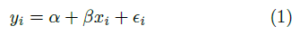
The optimal set of coefficients found for the linear regression’s equation is called the model. In our example, the linear regression equation involves only two variables: price and square footage. You can visualize the model and data points as follows, where square footage aligns on the x-axis, and the price aligns on the y-axis:

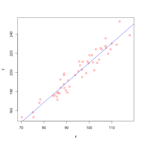
This prediction makes sense. The higher the price, the more square footage of the house. Of course, this is a relatively simple example. You could use a more complicated equation to predict the price of your house by looking at multiple predictors.

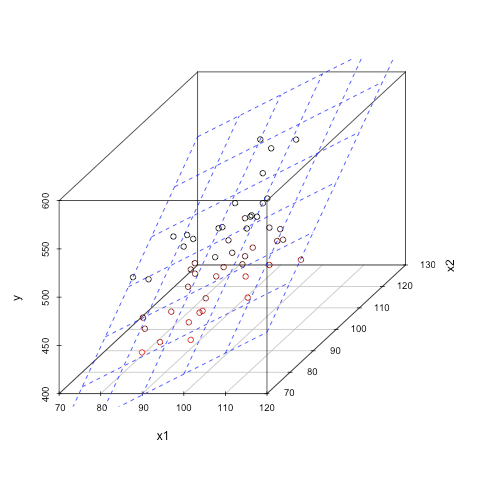
For example, imagine that in addition to considering square footage, you also want to consider the age of the home. Similarly, the objective is to find the set of coefficients for the following equation:

Because there are multiple predictors in this example, you also need multiple dimensions to visualize the model. With two predictors and one response, you could visualize your model as follows:

In Vertica, to employ linear regression, you must do the following:

1. Create training data.
2. Build your model.
3. Use your model on new data to make predictions.

The Prestige Data Set

Let’s take a look at an example using the Prestige data set. You can use this data set to find out how income is related to other variables. This data set is available online [2].

This example will show you how to load the data set and use the LINEAR_REG function in Vertica. You should use the example in your own Vertica database to better understand how the predictors impact the response. Can you figure out which predictor has the greatest impact on income?

The data set contains the following information:

• Name of occupation
• Education (in years)
• Income – Average income of incumbents in dollars in 1971
• Women – Percentage of incumbents who are women
• Prestige – The Pineo-Porter prestige score for the occupation, from a social survey conducted in the mid-1960s.
• Census – Canadian Census occupational code
• Type – Occupational type, where bc indicates blue collar, wc indicates white collar, and prof indicates professional, managerial or technical

The goal is to build a linear regression model using this data set that predicts income based on the other values in the data set. Then, you want to evaluate the model’s goodness of fit.

So, how do we choose which variables to choose for this model? We can eliminate the type column because Vertica does not currently support categorical predictors. The occupation and census columns contain a lot of unique values. These columns probably don’t make the most sense to predict income for our use case. So, let’s choose education, prestige, and women.

Note: In practice, if you need to consider a categorical predictor for training a linear regression model in Vertica, convert it to a numerical value in advance. There are several techniques for converting a categorical variable to a numeric one. For example, you can use one-hot encoding.

Load the Data

The following shows the table definition to store the prestige data set:
=> DROP TABLE IF EXISTS public.prestige CASCADE;
=> CREATE TABLE public.prestige (
occupation VARCHAR(25),
education NUMERIC(5,2), -- avg years of education
income INTEGER, -- avg income
women NUMERIC(5,2), -- % of woman
prestige NUMERIC(5,2), -- avg prestige rating
census INTEGER, -- occupation code
type CHAR(4) -- Professional & managerial (prof)
) -- White collar (wc)
-- Blue collar (bc)
-- Not Available (na)


To load the data from the prestige data set into the Vertica table, use the following SQL statement:
=> COPY public.prestige
FROM stdin
DELIMITER ','
SKIP 1
ABORT ON ERROR
DIRECT
;

Create a Linear Regression Model

Now, let’s use the Vertica machine learning function LINEAR_REG to create the linear regression model.

To create the model, run the LINEAR_REG function against the public.prestige table as shown. In this statement, income is the response, and the predictors are education, women, and prestige:
=> SELECT LINEAR_REG(
'prestige',
'public.prestige',
'income',
'education,women,prestige');

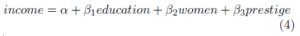
This statement is trying to identify the coefficients of the following equation:

After you create the model, use the SUMMARIZE_MODEL function to observe the model’s properties:
=> SELECT SUMMARIZE_MODEL('prestige');
SUMMARIZE_MODEL returns the following information:
SUMMARIZE_MODEL| coeff names : {Intercept, education, women, prestige}
coefficients: {–253.8390442, 177.1907572, –50.95063456, 141.463157}
p_value: {0.83275, 0.37062, 4.1569e–08, 8.84315e–06}

Using these coefficients, you can rewrite equation (4) to read:

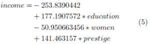
Finally, let’s explore how to measure how well the linear regression model fits the data, called goodness of fit. In Vertica, the PREDICT_LINEAR_REG function applies a linear regression model on the input table. You can read more about this function in the Vertica documentation.

Goodness of Fit

A common method used to test how well your linear regression model fits the observed data is the coefficient of determination. The coefficient is defined in the following equation:

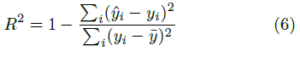
The coefficient of determination R2 ranges between 0 (no fit) and 1 (perfect fit). To calculate the coefficient of determination, use the Vertica RSQUARED function:
=> SELECT RSQUARED(income, predicted) OVER()
FROM ( SELECT
income,
PREDICT_LINEAR_REG (
prestige, women
USING PARAMETERS OWNER=’dbadmin’,
MODEL_NAME=’prestige’)
AS predicted
FROM public.prestige
) x ;
rsq | comment
-------------------+-------------------------------
0.63995924449805 | Of 102 rows, 102 were used ...

Note: The OWNER parameter will be deprecated in Vertica 8.1.

The evaluation of the coefficient of determination often depends on what area you are investigating. In the social sciences, a coefficient of 0.6 is considered quite good. [3]

When you evaluate a model, it is important to consider multiple metrics. A single metric could give you a good value, but the model itself may not be as useful as you need. It is important to understand the R-square value, as well as the other metrics, to evaluate the goodness of fit.

Keep an eye out for the next machine learning blog in our series!

References

[1] Prestige Data Set
[2] Canada (1971) Census of Canada. Vol. 3, Part 6. Statistics Canada.
[3] Julian J. Faraway. Linear Models of R, second edition. CRC Press, 2014
[4] Machine Learning for Predictive Analytics, Vertica documentation.
[5] Machine Learning Functions, Vertica documentation.
[6] Machine Learning for Predictive Analytics, Hands On Vertica.