


As an avid anthropology enthusiast, I often contemplate how we got to where we are today. We theorize we share common ancestors with apes, but what happened in between? Does a so-called ‘missing link’ exist somewhere, buried beneath the sands of time, waiting to be discovered? The truth is, we may never know. But, we can make educated guesses based on where we started and where we are now. We can fill in the gaps, so to speak, and analyze the path we took along the way to homo sapiens sapiens.
Evolutionary anthropology may seem a far cry from Big Data. But really, it’s not much different than the situation that businesses find themselves in today. Since data is often collected at random intervals, you might miss data that lies between the cracks. For example, when analyzing stock prices, you might find you don’t have an entry for the time between 10:01 am and 10:04 am. How can you analyze what happened in between? What does the ‘missing link’ in your data look like? Fortunately, you have a tool that anthropologists do not: Vertica time series analytics.
Time series analytics is a little-known, but very powerful Vertica tool. In Vertica, the TIMESERIES clause and time series aggregate functions normalize data into time slices. Then they interpolate missing values that fill in the gaps.
Using time series analytics is useful when you want to analyze discrete data collected over time, such as stock market trades and performance, but find that there are gaps in your collected data.
So, how does time series analytics work?
Gathering the Evidence: Using Time Series Aggregate Functions
First, let’s discuss how to define your time slice, or the time interval for which you want to produce output records. You do this using the TIMESERIES clause. Provide the TIMESERIES clause an INTERVAL slice time that determines when output records are produced. For example, if you specify one second, Vertica will produce an output record at every second and calculate values for seconds that do not have corresponding known values.
Now let”s look at the two time series aggregate functions. These functions determine which value within your defined time slice to output.
- TS_FIRST_VALUE: This function returns the value at the beginning of a time slice.
- TS_LAST_VALUE: This function returns the value at the end of the time slice.
Finding the Missing Links: Using Interpolation Schemes
Additionally, the time series aggregate functions allow you to specify an interpolation scheme, or a method of filling in missing data. You can choose between constant and linear.
The Constant Interpolation Scheme
The default constant interpolation scheme fills in missing data based on the last seen value so far. This means that the value at a constructed data point will match the value at the last known data point. In the graph below, the known data points are represented by a blue dot, and the interpolated values are represented by the blue stars. As you can see, the stars match the data points directly preceding them and don’t change until a new known value exists.
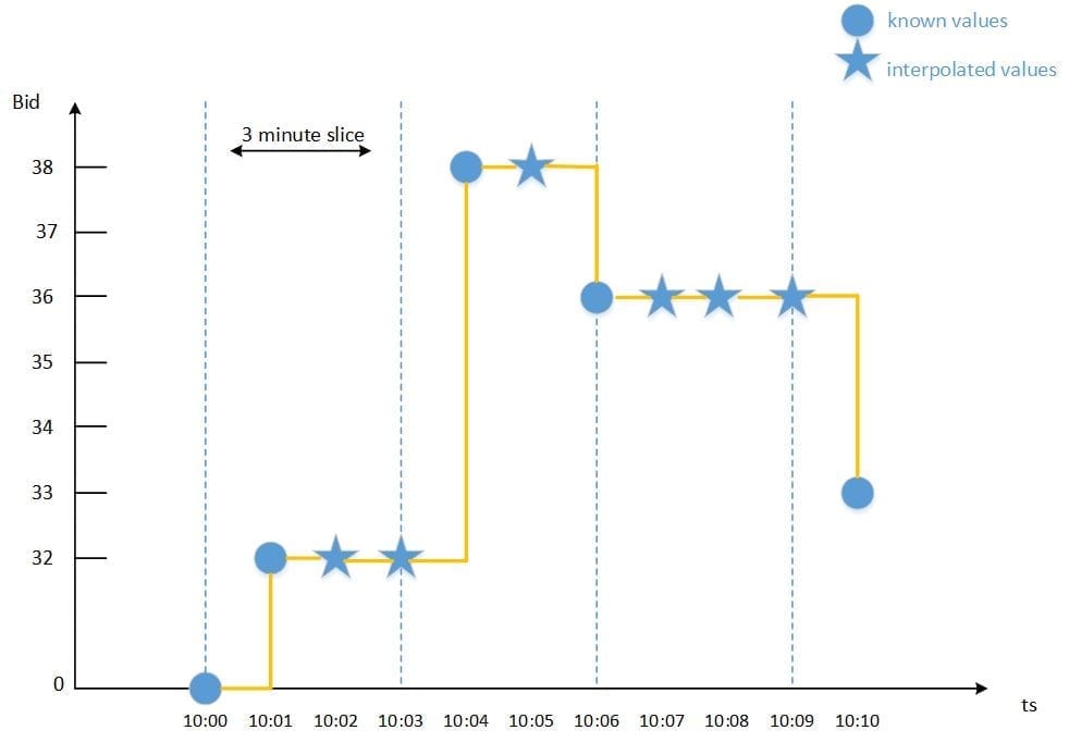
Constant interpolation scheme
The Linear Interpolation Scheme
The linear scheme interpolates values in a linear slope based on the specified time slice. In this case, a constructed data point value will fall between the values of the last known data point and the data point that follows the constructed point. In the graph below, the known data points are represented by a blue dot, and the interpolated values are represented by the blue stars. As you can see, the stars appear between two known data points along a linear slope.
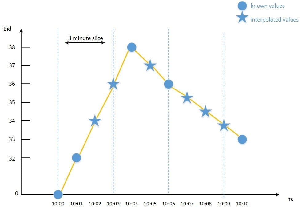
Linear interpolation scheme
Given the two time series aggregate functions, and the two methods of interpolations, we have four options for constructing our missing data points:
- TS_FIRST_VALUE with constant scheme, which fills in missing data points according to the last value seen so far, and returns the value at the beginning of the time slice.TS_FIRST_VALUE(value, ?’CONST’?)
- TS_FIRST_VALUE with linear scheme, which fills in missing data points according to a linear slope, and returns the value at the beginning of the time slice.TS_FIRST_VALUE(value, ?’LINEAR?’)
- TS_LAST_VALUE with constant scheme, which fills in missing data points according to the last value seen so far, and returns the value at the end of the time slice.TS_LAST_VALUE(value, ?’CONST’?)
- TS_LAST_VALUE with linear scheme, which fills in missing data points according to a linear slope, and returns the value at the end of the time slice.TS_LAST_VALUE(value, ?’LINEAR?’)
Applying Your Knowledge
As an example, let’s consider stock bid prices over time for company XYZ:
Table TickStore
| time | symbol | bid |
| 2014-09-30 10:00:00 | XYZ | 0 |
| 2014-09-30 10:01:00 | XYZ | 32 |
| 2014-09-30 10:04:00 | XYZ | 38 |
| 2014-09-30 10:06:00 | XYZ | 36 |
| 2014-09-30 10:10:00 | XYZ | 33 |
As you can see, there are time lags between several bids. Given these known values, how would you estimate a bid price at say 10:02?
Here, we use the TS_FIRST_VALUE function with both the constant and linear schemes. Both statements uses the TS_FIRST_VALUE function and divide the time into 1 minute slices using the TIMESERIES clause. The result is that we have a row for each minute within our defined data set, where the interpolated bid prices (shown in bold in the tables below) reflect the value at the beginning of each time slice. The first statement, reflected in the left table, uses the constant scheme, so each interpolated value is calculated from the last know value. The second statement, reflected in the right table, uses the linear scheme, so each value is interpolated according to a linear slope between known data points.
=> SELECT slice_time, symbol, TS_FIRST_VALUE(bid, 'CONST') AS first_bid FROM TickStore TIMESERIES slice_time AS '1 minute' OVER (PARTITION BY symbol ORDER BY time);
=> SELECT slice_time, symbol, TS_FIRST_VALUE(bid, 'LINEAR') AS first_bid FROM TickStore TIMESERIES slice_time AS '1 minute' OVER (PARTITION BY symbol ORDER BY time);
| Query Output (CONST) | Query Output (LINEAR) | ||||||||||||||||||||||||||||||||||||||||||||||||||||||||||||||||||||||||
|
|
How Will You Evolve?
While in this blog we used bid prices as an example, you can apply Vertica’s time series analytics to many problems. How will you use it?
For more information on time series analytics, see our documentation.
About the Author
Sarah Lemaire
Manager, Vertica Documentation