Using Vertica Machine Learning to Analyze Smart Meter Data

Machine learning and data science have the potential to transform businesses because of their ability to deliver non-obvious, valuable insights from massive amounts of data. However, many data scientist’s workflows are hindered by computational constraints, especially when working with very large data sets. While most real-world data science workflows require more than multiple cores on a single server to meet complexity, scale, and speed demands, many formal machine learning tools that are available today use single node machines with non-distributed algorithms. There is also a general knowledge gap when it comes to what machine learning on distributed systems looks like in practice, and how MPP distributed machine learning tools like Vertica can help in quickly generating insights from a very large amount of data.

Vertica is an advanced analytics MPP columnar database that is used by many of the leading data companies worldwide. Machine learning is built into the core of Vertica, making it extremely fast and easy to use with ANSI SQL99 compliant syntax that uses C++ under the hood to execute the algorithms. These functions run in parallel across multiple nodes in a Vertica cluster, delivering predictive analytics at speed and scale.

In this blog post, we demonstrate the application of some of Vertica’s machine learning capabilities using a data set by going through the steps of data exploration, preparation, model training, and evaluation.

The example used in this post is based on the Smart Meter data study performed by the Irish government. The data was collected from 1000 Irish homes, with kilowatt readings taken every 15 minutes, 24 hours a day over 1.5 years. Data collected included meter type, location, and weather information. We will use this information to predict high electricity usage based on historical use, residence type, location, date, time, and weather information.

Let’s take a closer look at the data. We pull the first few rows of the four tables using SELECT queries, such as the following:

=> SELECT * FROM consumption LIMIT 10;

The following tables show the readings from the homes:



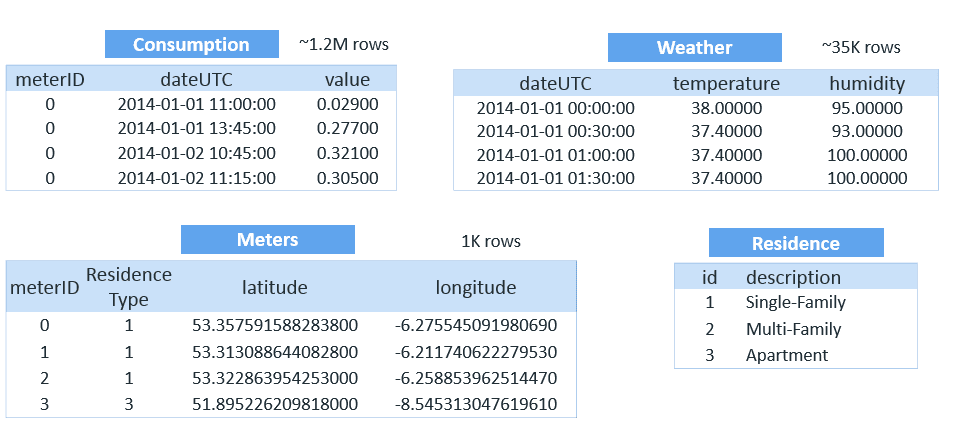
The consumption table is the largest, with more than one million rows.

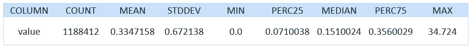
To further understand this information, we can use the SUMMARIZE_NUMCOL function to get a distribution of the meter readings (value in the following query) from the consumption table:

=> SELECT SUMMARIZE_NUMCOL (value) OVER() FROM user1.sm_consumption;

We get the following results:

Detecting Outliers

Now that we have a better understanding of the data, such as the mean consumption, we want to know more, such as why is the maximum consumption so high compared to the average? To do this, we can explore outliers in the data, using the DETECT_OUTLIERS function:

=> SELECT DETECT_OUTLIERS ('user1.sm_outliers', 'user1.sm_consumption'. 'value', 'robust_zscore' USING PARAMETERS outlier_threshold = 3.0);

Then, we can create a table to view the outliers:

=> CREATE TABLE user1.sm_consumption_outliers AS (SELECT c.*, CASE WHEN o.value IS NULL THEN 0 ELSE 1 END AS highusage FROM user1.sm_consumption c LEFT OUTER JOIN user1.sm_outliers o ON c.meterid = o.meterid AND c.dateUTC = o.dateUTC);

The following shows the results of the table:



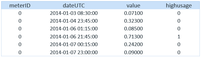
Now we have created a highusage feature using outlier detection.

Clustering Meter Locations

We can also use the machine learning function KMEANS to determine where there are geographic clusters of meters and let the function assign the various meters to cities by defining the city boundaries. Using this, we can better understand usage among residences in different cities.

First, let’s run the KMEANS function using the latitude and longitude. Every machine learning algorithm in Vertica has some optional parameters. In the following, we use the meterid as key columns to be passed to the output:

=> SELECT KMEANS ('user1.sm_kmeans', 'user1.sm_meters', 'latitude, longitude', 6 USING PARAMETERS key_columns = 'meterid');

With every Vertica machine learning prediction algorithm, there is also a corresponding APPLY or PREDICT function that applies the learnt model to a data set. The following shows a CREATE statement that uses the APPLY_KMEANS function to apply the model we just learnt to get the locationid column:

=> CREATE TABLE user1.sm_meters_location AS (SELECT meterid, residenceType, latitude, longitude, APPLY KMEANS (latitude, longitude USING PARAMETERS model_name = 'user1.sm_kmeans') AS locationid FROM user1.sm_meters);

The following shows the results of the table:



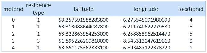
The following shows a visual representation of the different locationids:



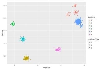
Now we have created a location feature using k-means. Depending on which city the meter reading was taken from, it may be helpful in predicting energy usage.

Understanding Weather and Consumption

Next, let’s take a closer look at how consumption and weather are related. It would make sense that in weather extremes (very hot or very cold), the consumption increases.

We’ll start by using a LEFT OUTER JOIN to join the consumption and weather data:

=> SELECT DISTINCT cdate, wdate, temperature, humidity FROM (SELECT c.meterid, c.dateUTC AS cdate, w.dateUTC AS wdate, w.temperature, w.humidity, c.value FROM user1.sm_consumption c LEFT OUTER JOIN user1.sm_weather w ON c.dateUTC = w.dateUTC ORDER BY cdate) a ORDER BY 1 LIMIT 10;

The following shows the output of this query:



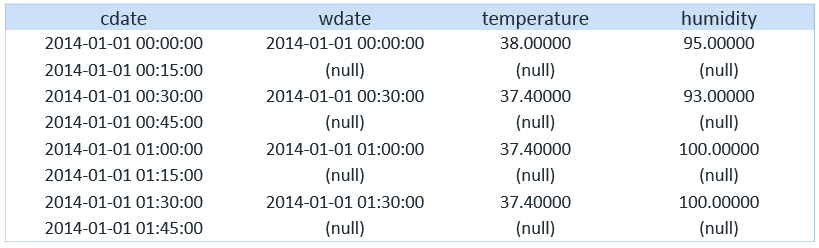
Weather reading is taken every 30 minutes, and kilowatt readings were taken every 15 minutes. Whenever the readings do not align, we get a null value.

Then, using the TIMESERIES clause, we can fill the gaps in the data:

=> CREATE TABLE user1.sm_weather_fill AS SELECT ts AS dateUTC, TS_FIRST_VALUE(temperature, 'LINEAR') temperature, TS_FIRST_VALUE (humidity, 'LINEAR') humidity FROM user1.sm_weather TIMESERIES ts AS '15 minutes' OVER (ORDER BY dateUTC);

The following shows the output:



Finally, bring all the tables together for modeling by creating one flat table. This also uses a case statement to divide the data randomly into test and train data sets, with 30% and 70% of the data, respectively:

=> CREATE TABLE user1.sm_flat_temp AS SELECT c.meterid, r.id, l.locationid::varchar, dayofweek(c.dateUTC) AS dow, month(c.dateUTC) AS moy, case when month(c.dateUTC) >= 3 and month(c.dateUTC) <= 5 then 1 else 0 end as 'Spring', case when month(c.dateUTC) >= 6 and month(c.dateUTC) <= 8 then 1 else 0 end as 'Summer', case when month(c.dateUTC) >= 9 and month(c.dateUTC) <= 11 then 1 else 0 end as 'Fall', hour(c.dateUTC) as hod, case when hour(c.dateUTC) >= 6 and hour(c.dateUTC) <= 11 then 1 else 0 end as 'Morning', case when hour(c.dateUTC) >= 12 and hour(c.dateUTC) <= 17 then 1 else 0 end as 'Afternoon', case when hour(c.dateUTC) >= 18 and hour(c.dateUTC) <= 23 then 1 else 0 end as 'Evening', w.temperature, w.humidity, c.highusage, case when random()<0.3 then 'test' else 'train' end as part FROM user1.sm_consumption_outliers c inner join user1.sm_meters_location l on c.meterid = l.meterid inner join user1.sm_residences r on l.residenceType = r.id inner join user1.sm_weather_fill w on c.dateUTC = w.dateUTC;

Use One Hot Encoding

Now that we have all the data in one table, we want to be able to query that data. To do so, we need all the data to be in numerical format. We also need to convert the categorical data into dummy/indicator columns. We can do that using one hot encoding, which will create dummy columns from a given column in Vertica:

=> SELECT ONE_HOT_ENCODER_FIT ('user1.sm_onehot', 'user1.sm_flat_temp', 'id, locationid, dow');

Then, create a table for this data:

=> CREATE TABLE user1.sm_flat AS (SELECT APPLY_ONE_HOT_ENCODER(* USING PARAMETERS model_name = 'user1.sm_onehot', drop_first = 'true') FROM user1.sm_flat_temp);

Balance the Training Data

Next, we must balance the training data set we created:

=> SELECT BALANCE ('user1.sm_flat_train_balanced_view', 'user1.sm_flat_train', 'highusage', 'hybrid_sampling');

Then, create a table for this data:

=> CREATE TABLE user1.sm_flat_train_balanced AS (SELECT * FROM user1.sm_flat_train_balanced_view);

Train the Models

Next, we can train the models using two different algorithms: logistic regression and SVM for classification. Logistic regression is a binary classification algorithm. It produces a linear model that estimates the class probability. SVM is also a binary classification algorithm that performs L2 regularization by default, thereby controlling overfitting.

Let’s start with logistic regression:

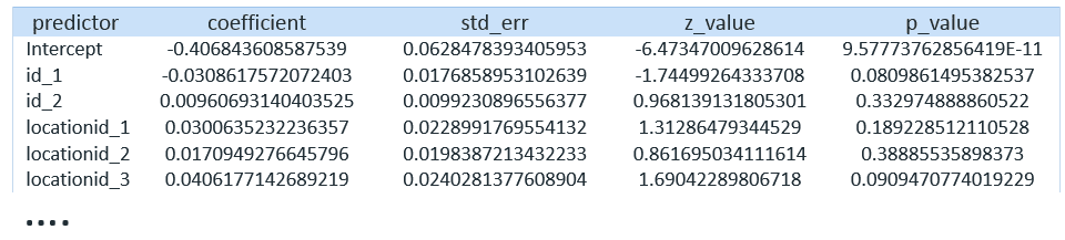
=> SELECT LOGISTIC_REG ('user1.sm_logistic', 'user1.sm_flat_train', 'highusage','id_1, id_2, locationid_1, locationid_2, locationid_3, locationid_4, locationid_5,dow_1, dow_2, dow_3, dow_4, dow_5, dow_6, Spring, Summer, Fall, Morning,Afternoon, Evening, temperature, humidity');

Then, we can get a summary by calling GET_MODEL_ATTRIBUTE and view the details for each location:

=> SELECT GET_MODEL_ATTRIBUTE (USING PARAMETERS model_name = 'user1.sm_logistic', 'attr_name = 'details');

Let’s do the same with SVM:

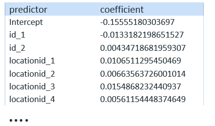
=> SELECT SVM_CLASSIFIER ('user1.sm_svm', 'user1.sm_flat_train', 'highusage','id_1, id_2, locationid_1, locationid_2, locationid_3, locationid_4, locationid_5,dow_1, dow_2, dow_3, dow_4, dow_5, dow_6, Spring, Summer, Fall, Morning,Afternoon, Evening, temperature, humidity');

And we can get a similar summary using GET_MODEL_ATTRIBUTE:

=> SELECT GET_MODEL_ATTRIBUTE (USING PARAMETERS model_name = 'user1.sm_svm', 'attr_name = 'details');

Evaluation

Finally, we can use cross validation to evaluate the models. We apply cross validation with both the algorithms with a k value of 5. This enables us to see whether logistic regression or SVM performed better:

=> SELECT CROSS_VALIDATE ('logistic_reg', 'user1.sm_flat_train', 'highusage', 'id_1, id_2, locationid_1,locationid_2, locationid_3, locationid_4, locationid_5, dow_1, dow_2, dow_3, dow_4, dow_5, dow_6, Spring, Summer, Fall, Morning, Afternoon, Evening, temperature, humidity' USING PARAMETERS cv_fold_count= 5, cv_model_name='user1.sm_cv_lg', cv_metrics='error_rate'); => SELECT CROSS_VALIDATE ('svm_classifier', 'user1.sm_flat_train', 'highusage', 'id_1, id_2, locationid_1, locationid_2, locationid_3, locationid_4, locationid_5, dow_1, dow_2, dow_3, dow_4, dow_5, dow_6, Spring, Summer, Fall, Morning, Afternoon, Evening, temperature, humidity' USING PARAMETERS cv_fold_count= 5, cv_model_name='user1.sm_cv_svm', cv_metrics='error_rate');

Then, we can look at the evaluation results by using GET_MODEL_ATRIBUTE:

=> SELECT GET_MODEL_ATTRIBUTE (USING PARAMETERS model_name = 'user1.sm_cv_lg', attr_name = 'run_average'); => SELECT GET_MODEL_ATTRIBUTE (USING PARAMETERS model_name = 'user1.sm_cv_svm', attr_name = 'run_average');

Which algorithm performed better?



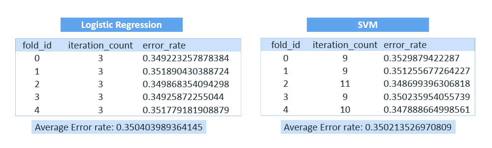
While they were both very close, with a low error rate, ultimately SVM performed slightly better than logistic regression.

For more information, see Machine Learning for Predictive Analytics in the Vertica documentation.